Scaling Laws and Chinchilla
In this post I explain what I learned from the Google Deepmind scaling laws paper “Training Compute-Optimal Large Language Models”.
Setup
The intention of the paper is to find out how to train the most effective language model given a budget. Instead of measuring the budget in dollars, they measure it in floating point operations (FLOPs). FLOPs is the natural unit for a problem like this since dollars per FLOP tends to decrease so much over time.
The fundamental question of “What is the most intelligent system we can create given a budget?” is hard to answer. Across all combinations of model architectures and modalities (text, audio, video, physical systems, etc.) there are just so many variables get right. It seems like there are many viable approaches! Nevertheless the paper focuses on dense transformer language models and plays with the following parameters:
- The number of model parameters.
- The amount of data that a given model is trained on.
The conclusion is: as the budget increases the number of model parameters and the amount of data should be increased in about the same proportion. This conclusion is different than the widely accepted thinking at the time which said that as budget increased, the number of model parameters should increase much more quickly than the amount of data the model is trained on.
After detailing their analysis they demonstrate their results concretely by training a model they call Chinchilla. By training on significantly more data Chinchilla outperforms much bigger models (4x bigger!) on a variety of metrics.
Given the significant cost of training large language models (see below) and their demonstrated importance to society, answering these kinds of basic questions is important.
A note on counting FLOPs and building intuition
Counting flops
There’s a nice result which says that training a transformer model with $N$ parameters on $D$ tokens (units of data) requires about
$$ \mathrm{FLOPs} \approx 6 N D $$
We get this by counting FLOPs for matrix multiplies in the forward and backward passes.
This equation will be used repeatedly throughout. A helpful corollary to keep in mind is that every model size sets a minimum number of FLOPs required to run a single training step. Even if we have a huge model, we can’t teach it anything if we don’t have the budget!
A few back of the envelope calculations
They train Chinchilla on a budget of about $10^{24}$ FLOPs. It’s hard to have intuition for a number like that. How much money might that cost? How much energy? What is that similar to? Let’s try to get a handle on some of these things before getting into the paper.
Let’s assume training is taking place on Nvidia Grace Hopper GPUs (GH200 NVL2). Looking at the chip data sheet for TF32 Tensor Core performance let’s assume that each GPU is doing 1000 TeraFLOPS (i.e., $10^{15}$ FLOPs/s) all the time during training. Also from the data sheet let’s assume each GPU requires 1000 Watts of power.
Time:
For a single GPU training would take
$$ T_{\mathrm{single}} = \frac{10^{24}FLOPs}{10^{15}FLOPs/s} = 10^9s \sim 32 \hspace{1mm}\mathrm{years} $$
–so clearly, training must be distributed across many GPUs. Suppose training goes for about 3 months (i.e., $7.88 \times 10^6s$).
GPU count for 3 months of training:
$$ GPU_{3 -\mathrm{month}} = \frac{10^{24} FLOPs}{10^{15}FLOPs/s * (7.88 \times 10^6 s)} \approx 127 $$
It’s hard to know precisely what it would cost to buy a GH200 NVL2 chip. Renting something like it on Lambda Labs costs about $1.50/hr. So having 127 for 3 months would cost about $400k. Surely there’s volume discounting and so on. I also haven’t dug into the exact specs of the instances on Lambda Labs, but it’s a first estimate.
Power: For reference 1000 Watts is about the power demanded by a window AC unit. Having 127 of these GPUs running requires 127,000 W ↔ 127 kW. Over the course of three months of training that leads to about
$$ \mathrm{Energy}_{3-\mathrm{month}} \sim 2.8 \times 10^5 \hspace{1mm}\mathrm{kWh} $$
Some quick searching shows, on average, a hospital uses about $77 \times 10^5$ kWh of energy from electricity per year (31 kWh/sq. ft @ 247k sq. ft). So in the three months for training
$$ \mathrm{Energy_{127 -GPU}} \sim 2.8 \times 10^5 \hspace{1mm} \mathrm{kWh} $$ $$ \mathrm{Energy_{hospital}} \sim 19 \times 10^5 \hspace{1mm} \mathrm{kWh} $$
So training the network was like running a wing of a hospital. Should be a good model!
The key figures
Figure 1: Increase the number of model parameters as budget increases
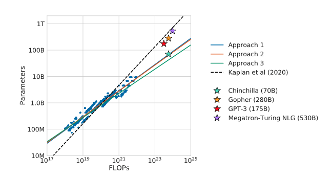
By how much? The colored solid lines are from their various modeling approaches. The dashed black line shows predictions from another group who investigated the problem. The major point is previous thinking called for too many parameters as FLOPs budget increases. The three stars near the top line indicate that the field was generally following the results of Kaplan and others. The authors’ model Chinchilla is 2.5 to 7.5 times smaller than those models, yet it outperforms them.
Note: Smaller models also mean they fit on less expensive hardware and are cheaper to use in the wild!
Table 1: Train on more tokens
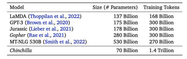
Models at the time had a huge number of parameters but trained on a small amount of data relative to Chinchilla.
Figure 2: Approach 1 - Fix model size and train on more tokens
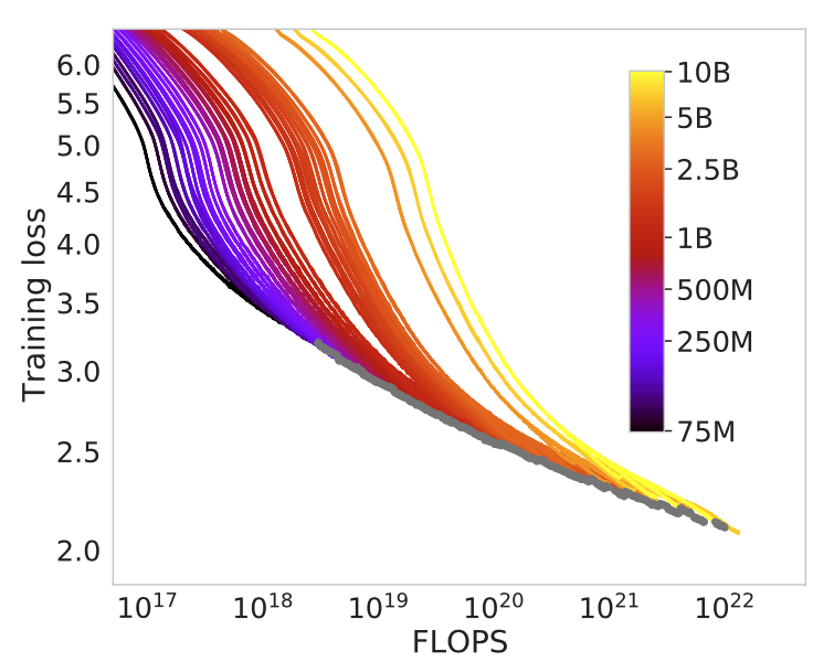
The authors consider a family of models ranging in size from 70M to 10B parameters. They train each model four times increasing the amount of data, and hence the number of FLOPs, they train on each time.
They use this data to extract the number of model parameters that give the minimum training loss for a given FLOP count. From this they fit a power law for the optimal number of model parameters $N_{opt}$ given a computational budget $C$ (measured in FLOPs):
$$ N_{opt} = A C^a $$
Recall the approximation $\mathrm{FLOPs} \approx 6 N D$. With this approximation we can use the fit for $N_{opt}$ to fit $D_{opt}$ (the optimal number of tokens to train on).
$$ C = 6 N_{opt} D_{opt} \implies D_{opt} = \frac{C}{6 N_{opt}} = \frac{1}{6A} C ^{1-a} $$
Since we typically care about ratios, the most important part of the fit is the scaling exponent $a$ which they find to be $a = 0.5$.
$$ N_{opt} \sim C ^{0.5}, \ D_{opt} \sim C ^ {0.5} $$
What does it mean? As the computational budget increases by a factor of 10, the number of model parameters and the number of tokens we train on should each increase by a factor of $\sqrt{10} \approx 3$.
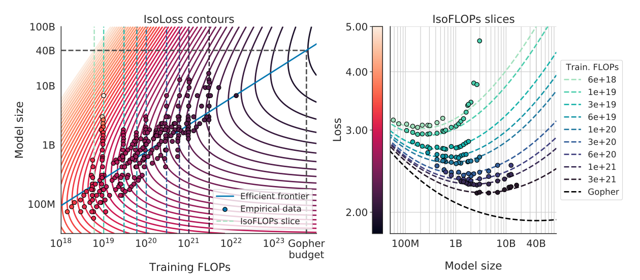
Figure 3: Approach 2 - Fix the number of flops and investigate training loss
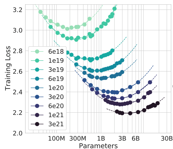
Each curve is what they call an “IsoFLOP curve” where all points have the same number of FLOPs. This is a nice way of doing things. Fix the number of FLOPs, train models of various sizes to that FLOP count, and see what loss results.
The results are fairly intuitive. In the top left we have curves with few FLOPs, few model parameters, and relatively high training loss. Remember $\mathrm{FLOPs} \approx 6 ND$ so large models can’t even be trained on a low FLOP count! As we move to the bottom right we have high flop count, large models, and relatively low training loss.
Basically what this is saying is that we can’t just use a bigger model to lower the loss for a fixed FLOP count. Instead, we need to balance model size with being able to take a sufficient number of training steps ↔ learn from enough data. Same story as in approach one.
They fit a parabola to each curve to find the number of model parameters which minimizes the loss for a given FLOP count. From this data they are able to fit a function to project the optimal number of parameters for a given FLOPs budget
$$ N_{opt} = A C^a $$
with this method they find $a = 0.49$. As before, plugging this relation into our $\mathrm{FLOPs} \approx 6 N D$ formula, we get
$$ N_{opt} \sim C^{0.49}, \ D_{opt} \sim C ^ {0.51} $$
Figure 4: Approach 3 - Model the loss and fit a function
These figures are kind of a mess but again the approach is nice. The authors basically say “We have all of these training runs where we know the loss for a given model size and amount of data trained on. Why not just fit a function to all of that?” The authors model (i.e., they choose this form!) the loss as a sum of three terms
$$ L(N, D) = E + \frac{A}{N^\alpha} + \frac{B}{D^\beta} $$
The term $E$ corresponds to the “entropy” of natural text. I think of it as the inherent unpredictability of what will come next in language. The second term $\frac{A}{N^\alpha}$ captures the intuition that the loss should decrease as the model gets bigger, independent of anything else. The final term $\frac{B}{D^\beta}$ captures the intuition that as we train on more data the training loss should go down, independent of anything else.
So, to fit this function $L(N, D)$, they have to fit all five of these parameters $\set{E, A, B, \alpha, \beta}$. They use a method where they minimize the “Huber” loss between the predicted loss and the observed loss for all their training runs. The point is that it’s a method to find the parameters which fit the data the best.
If you minimize the loss by constraining $\mathrm{FLOPs} = 6 N D$ you end up with equations saying
$$ N_{opt} \sim C^{0.46}, \ D_{opt} \sim C^{0.54} $$
These scaling exponents are not quite equal to, but are very similar to, the exponents from the other two approaches.
The curves in the “IsoLoss contours” plot show how we can change the model size and flop count and keep the loss fixed. The “efficient frontier” line intersects each IsoLoss curve at the point where it minimizes the FLOPs count (minimize our budget for a given loss!). So, for a given budget, we just go vertically up until we hit the efficient frontier. That point will tell us both what our training loss is predicted to be and what model size we should use to get there.
The second plot shows IsoFlop curves (i.e., same number of Flops for all points on the curve) and how the loss changes (y-axis) as the number of parameters increases. The color scheme of the combined figure is a bit confusing but this is my interpretation. We can see that the fit is not perfect, especially in the low FLOPs regime. Note how the data points depart pretty far from the IsoFLOP slice for the $10^{19}$ training FLOPs line. The overall fit looks pretty good though.
Tables - Chinchilla vs Larger models
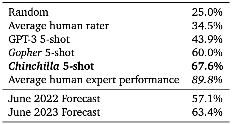
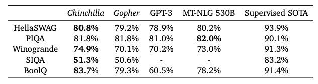
Finally the authors test their hypotheses by training the Chinchilla model. Note it’s four times smaller than Gopher. I haven’t explained the scores but the idea is to just show Chinchilla outperforms across a wide range of tasks. It’s also interesting to note that the models performed better than expert forecasts (5 shot test).
Summary
Big models are expensive to train both financially and energetically. It’s wise to optimize them for size. Not only do small models cost less to train, they cost less to use. This paper describes a method for finding the proper size of a language model given a budget. They use their method to show that state of the art models at the time were way too big. They test their hypothesis by training a relatively small model which indeed does outperform.
The authors also state that the same methodology can be used to determine the right size for models in other domains. For example, they suggest the same methods can be used to figure out how big a voice or video generation model should be. That seems reasonable, and I know similar studies are done before training large models today.
Ultimately we want to build the most helpful technologies with the resources we have. This paper helps us take a step in that direction!